Logica Capital commentary for the month ended October 2021.
Q3 2021 hedge fund letters, conferences and more
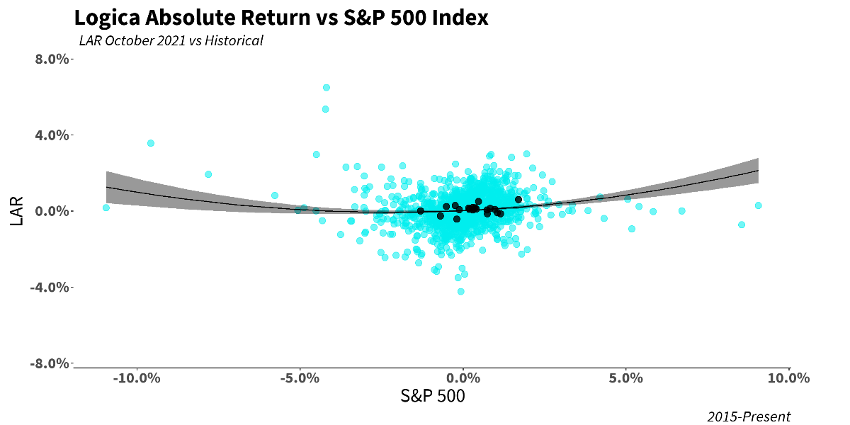
Logica Absolute Return (LAR) – Upside/Downside Convexity – No Correlation
- Tactical/dynamic balanced Put/Call allocation – Straddle
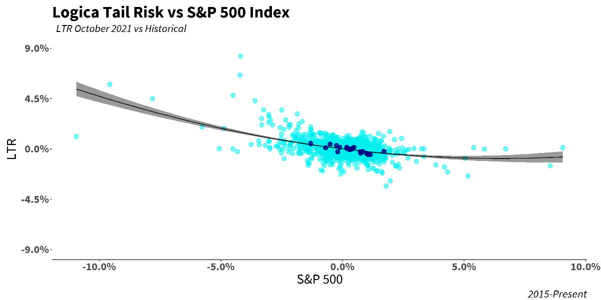
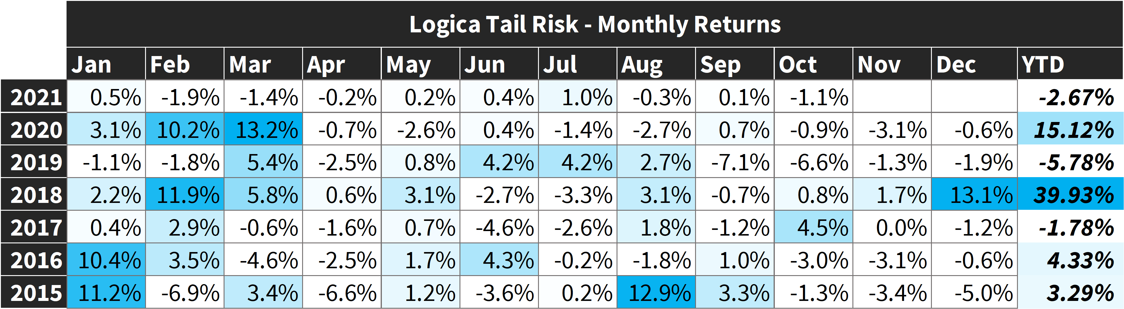
Logica Tail Risk (LTR) – Max Downside Convexity – Strong Negative Correlation
- Tactical/dynamic downside tilted Put/Call allocation – Ratio Straddle
Summary
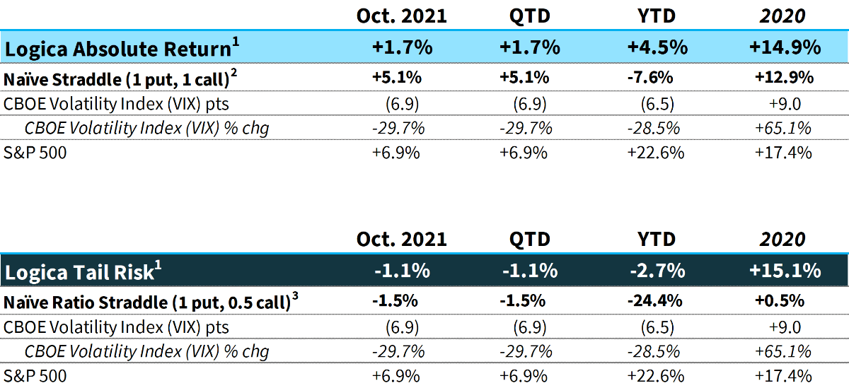
Following its first significant losing month in 2021, the S&P 500 rocketed straight back to all-time highs. In the process, the CBOE Volatility Index (VIX) recorded its lowest close of the year, and lowest close since February 19th, 2020. Logica’s strategies were able to largely withstand the substantial volatility crush due to gamma scalping, outperformance in our growth/momentum models, and a healthy contribution from our macro portfolio.
1 Returns are Gross of fees. LAR Fund +1.58% (net), LTR Fund -1.21% for October 2021
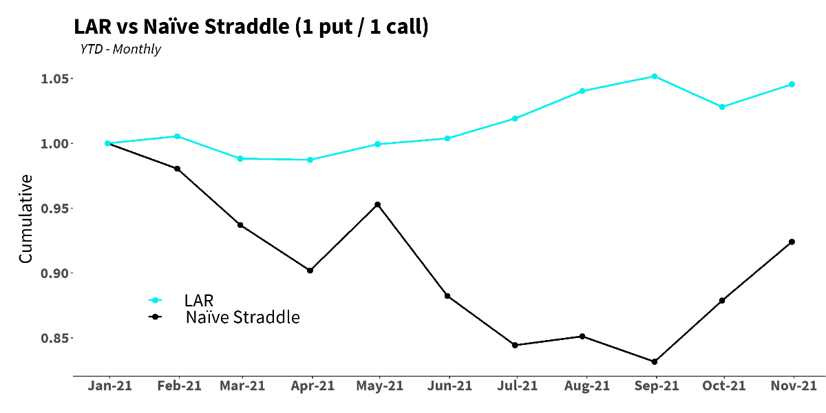
2 Naïve Straddle Return: a 1.5 month out, S&P 500 at-the-money put and call bought on the final trading day of prior month and sold on the final trading day of current month. This return on premium is divided by a factor of 6 to be comparable to Logica’s typical AUM-to-premium ratio.
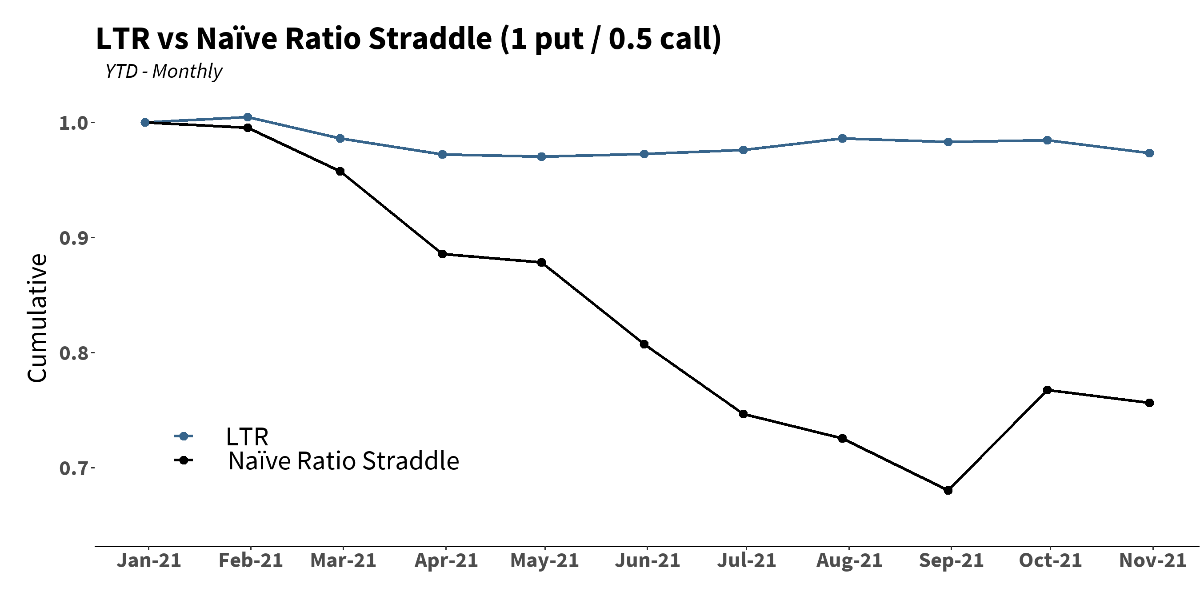
3 Naïve Ratio Straddle Return: a 1.5 month out, S&P 500 at-the-money put and at-the-money call (divided by 2) bought on the final trading day of prior month and sold on the final trading day of current month. This return on premium is divided by a factor of 6 to be comparable to Logica’s typical AUM-to-premium ratio.
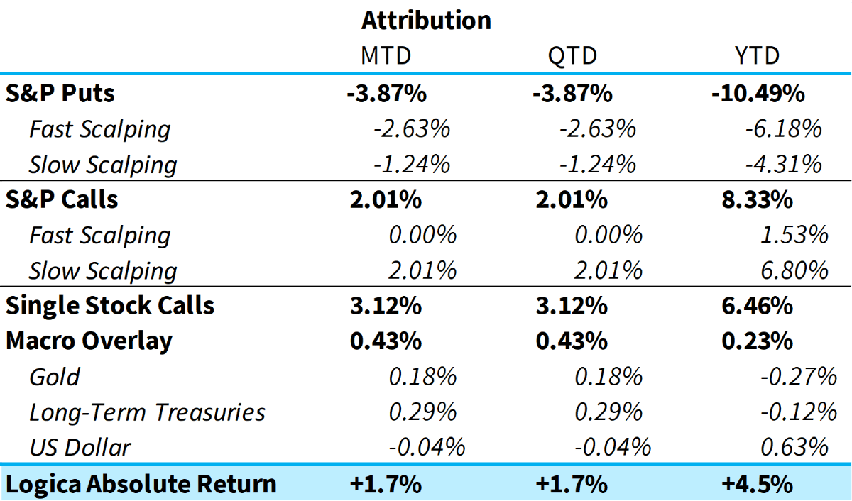
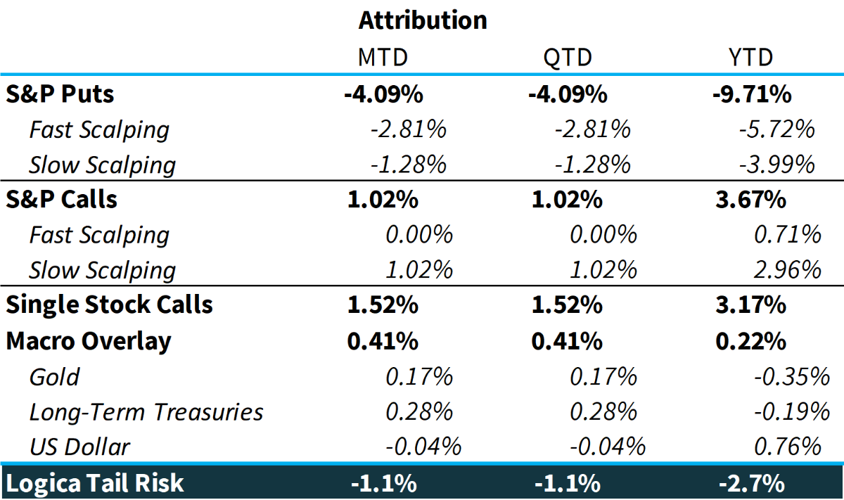
Commentary & Portfolio Return Attribution
“It’s better to go slow in the right direction than to go fast in the wrong direction.”
– Simon Sinek
Well, the Great Correction of 2021 didn’t last very long. Despite getting whipsawed with last month’s downside head-fake action, we were happy to see our models achieve quite the opposite in October, behaving with the precision that we aim for. Because of the lack of intra-month volatility, our fast scalping modules had minimal opportunities to positively contribute, but typically this is where the slower scalping modules shine (relatively speaking), as we see above.
In fact, October is a perfect illustration of the difference between our “fast” and “slow.” As markets exhibit varying speeds of swinging to and fro – conceptually, at different frequencies – any successful trading program, in our view, should either have the abiltiy to modify its cadence or else operate in both. In building our portfolio, we decided to bifurcate the “fast” and “slow,” rather than increasing/decreasing cadence within a single module, specifically so that we can get a better understanding of the behaviors, and further optimize under each frequency. October exemplified this difference, demonstrating the value of “slow” scalping during the market’s continued upward grind.
But does this necessarily mean that “fast” got it wrong? In some sense, yes, but in another sense, certainly not. It obviously got it wrong in that it took upside off the table too quickly given how much more the move was going to extend on this particular occasion. But it got it right for every one of those other times that an extended move is in fact already an extended move, which tends to be the case more often. Broadly, we prefer to bet on the higher odds when it comes to profit-taking as not doing so can leave us vulnerable, versus those few occasions when taking profits too early was the “wrong” thing (and of course, only in our “fast” scalping module).
Single Stock Calls were a significant outperformer this month, owing primarily to strong moves in our growth/tech related positions. Our focused diversifier module, focused mostly on anti-momentum/value, was still a solid contributor to the upside, but only half as much as the momentum module. Clearly, October saw a rotation into the favored tech sector, where once again some of the more “high flying” positions got a chance to shine.
Our Macro Overlay also logged a great October, driven by outperformance in long-term treasuries. As we’ve mentioned previously, this module has been a focus of our research over recent months, especially given the rate headwinds we expect going forwad. That said, we aren’t ready to communicate our findings quite yet (nor are we ready implement in live trading, as we desire greater levels of empirical rigor than we have at present), but are looking forward to nearing some innovation along these lines, or at the very least some value-added iterations.
“From naïve simplicity we arrive at more profound simplicity.” – Albert Schweitzer
A final thing to touch on with respect to October: a straddle-like exposure will typically excel during a strong trending environment. As we’ve delved into before, this is simply because one side of the straddle (this month, the Put side) deteriorates to be nearly worthless in value, while the other side (this month, the Call side) continues appreciating. Simply: Puts lose delta, and Calls gain delta. Our exposure was able to take advantage of this natural delta accumulation. However, and importantly, it does so in a protected fashion.
Because we are hyper-focused on risk management at the core of our trading philosophy, we trade regularly (in fact, daily) in aims to keep this accumulating exposure in check rather than simply letting it run wild. In the extreme opposite, a naïvely implemented straddle (that we have chosen as a benchmark) does let the exposure run wild. And therefore, the naive implementation had a fantastic period; however, only if one is merely focused on the Return side of the Risk/Return equation.
What do we mean by this? What’s critical to note here is that toward the end of October, the naïve straddle was long about 80 deltas (a -10 delta Put, and a 90 delta Call), making the naïve implementation essentially long the market, and terrifically downside exposed. While it’s easy to look back and see that the market just kept climbing, if it had even 1 or 2 days of reversion, or a more violent move down of multiple percent on any random calendar day toward the end of the month, the naïve straddle would have gotten crushed. Accordingly, in the naïve format, one is positioned more and more in “hope” mode as a month marches forward; an unacceptable arbitrariness in portfolio management.
On the other side of the coin, a dynamically hedging straddle effectively “chases” the accreting return with risk mitigation, with an aim of reducing that delta spread such that whenever that reversal day (or two, or three, or…) arrives, it can begin to participate in that other direction. This balance – letting it run vs. hedging it away – is always the challenge with managing a dynamic exposure whose profile changes with the underlying market (as opposed to owning an equity position, which is always delta 1.00). However, as the old adage goes, with great challenge comes great reward, and our reward is the crisis convexity that comes along with tightly managing optionality.
“Details create the big picture” – Sandy Weill
To that end, we thought it would be valuable to share how our crisis payoff structure has improved over recent months. In relation to some of our letters earlier this year where we discussed managing around the bear market in implied volatility coming off 2020 (the “IV crush”), we were happy to see more “normal” levels as we moved further into 2021. Moreoever, as implied volatility has moved even lower over the course of 2021 (on various occasions, VIX dropping down to the 14-15 range, nicely below the S&P’s historical average volatility of approximately 16), we have been able to meaningfully increase our average inventory of Puts (while still of course trading that Put exposure along the way). As a reference, here is our Put inventory YTD, where alongside our trading activity that dynamically modulates this inventory, the general trend of increasing Puts held is quite clear.
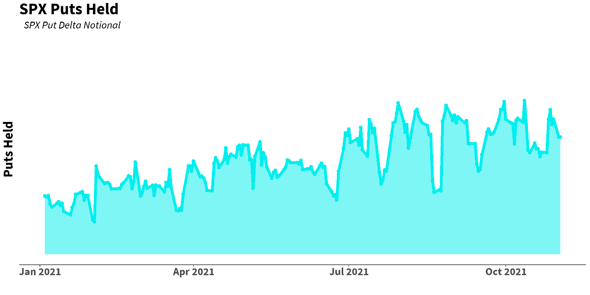
With this in mind, we continue to improve our overall positioning, and exposure, for a substantive downside event. While our inventory at any single moment may fluctuate given our trading/scalping approach, our overall trend toward increasing exposure is an important, big picture takeaway.
Finally, here’s a look at the naïve straddle benchmarks for the year:
Scatter plots for October are as expected:
Logica Strategy Details
Note: We have comprehensive statistics and metrics available for our strategies, but only include a select few to highlight what we believe is our most valuable contribution to any larger portfolio.
If you would like to learn more about our strategies, please reach out to:
[email protected]
Follow Wayne on Twitter @WayneHimelsein
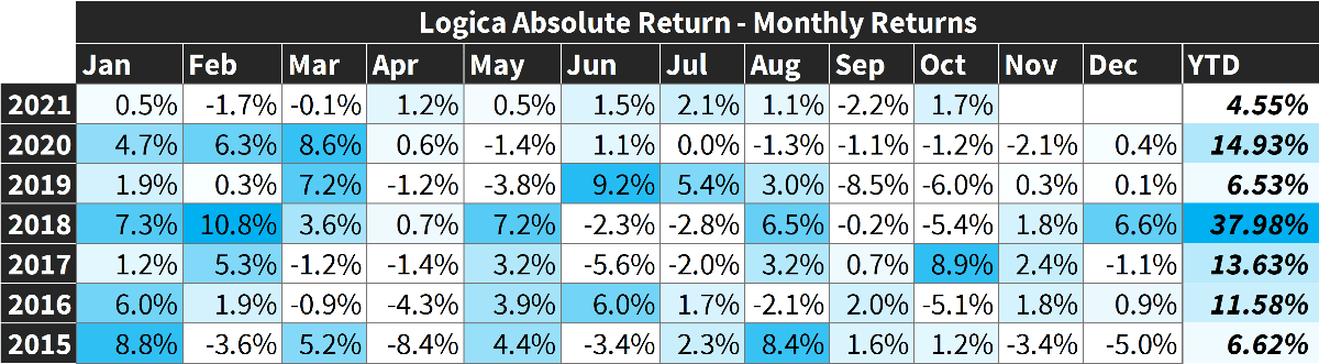
Logica Absolute Return
2015-2019 stats & grid, reconstitution of live sub-strategies normalized to 16% annualized volatility
2005 to present growth of $1000 chart, simulation
Jan 2020 live
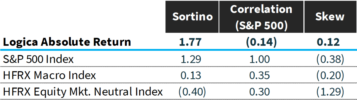
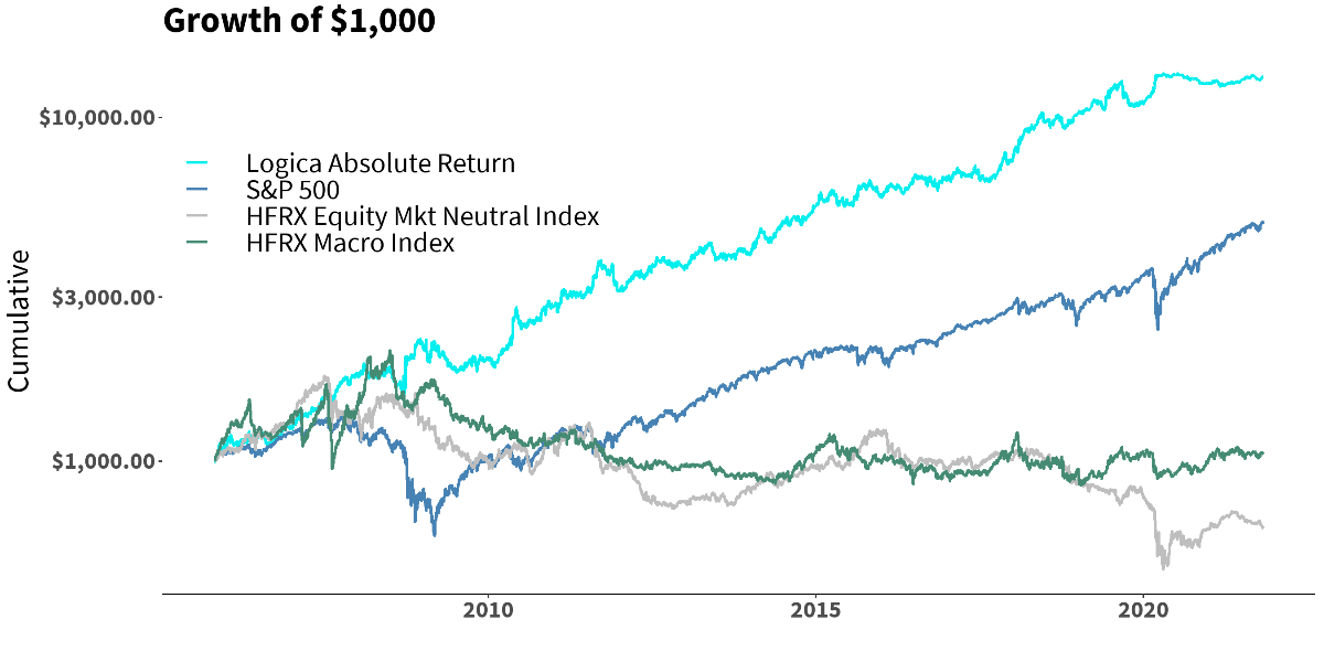
*HFRX Indices have been scaled up to 15% annualized volatility to be comparable to LAR and S&P 500.
Logica Tail Risk
2015-2019 stats & grid, reconstitution of live sub-strategies normalized to 16% annualized volatility
2005 to present growth of $1000 chart, simulation
Jan 2020 live
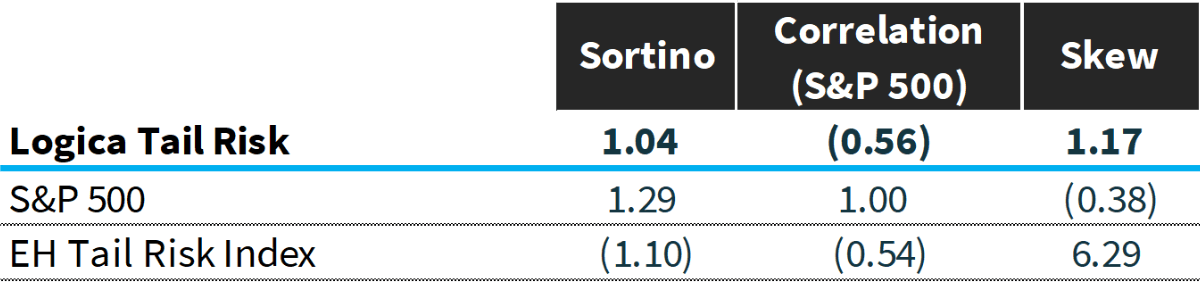
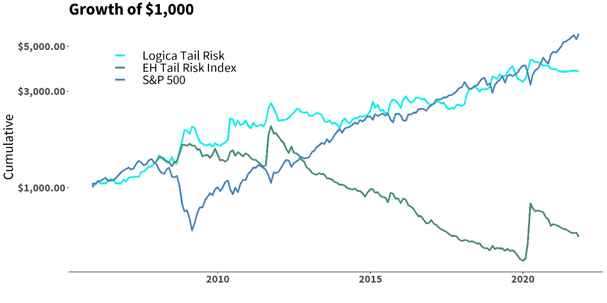
*EHTR Index has been scaled up to 17% annualized volatility to be comparable to LTR.