We have written several pieces on the famous small-firm or size effect, the two most important (IMHO) being our study of the interaction of size and quality and a fairly comprehensive survey of all things size. This note focuses on daily instead of the longer-horizon data studied in these other papers and, while not changing the overall story, this leads to a powerful illustration of what’s going on in small stocks.
The State of Play
Before I turn to the daily data, it’s important to step back and summarize what we’ve already said about the size effect – partly because there still seems to exist some confusion (some of that is clearly on us!). 2 , 3 First off, we do not reject that historically small firms have had larger average returns than big ones (though the victory is pretty meager). Some think that shows the existence of the size effect. They’re wrong. Basically, what we have all done in finance since the 1960s is not just look at average returns but average returns net of some “factor exposures.” That is, if you made extra money in small stocks but only because you were more exposed to some other known source of return, that may mean the real effect is this other source and not size. It’s often debatable what factors for which to adjust. Were these factors known ex ante? Do they have an economic story or might they be the result of data mining? These can be difficult issues for some factors. But, since the size effect was first studied in the early 1980s, one factor has always been adjusted for in any reasonable work. That factor is market beta.
If small stocks outperform, but it’s solely because of having higher market betas, nobody in modern finance would (or should) call that a small firm effect. The original work on the size effect back in the early 1980s didn’t miss this, finding that small beats large by more than market beta could explain. 4 , 5 But, the near 40 years since those findings have not been kind – both in realized returns and in re-examination of the original finding. A series of cumulative challenges, many of which we have summarized (though I’ll only address a subset here), all have reduced the historic “net of market beta” return to small vs. large, ultimately leaving nothing. Two of the main ones are 1) the original results, through no fault of their own, exaggerated the size effect as the databases at the time overstated the returns to small stocks. You get a smaller size premium today if you run the exact same tests over the exact same databases (updated and improved to fix errors, many of which were more common among small stocks) over the exact same time periods as the original work. 6 And 2) the apparent outperformance of small versus large caps after adjusting for market beta in the original work was biased by misestimated betas due to liquidity differences. Accounting for this misestimation removes the last vestige of a size effect.
Small stocks are less liquid, often far less liquid (particularly in the microcaps, which drive a large amount of the simple size effect). There are many ways to adjust for this, for instance adding explicit additional “liquidity factors” to regressions. But I will focus on the simplest of all that we have studied. In coming up with the market beta of small and large stocks, one simple way to adjust for illiquidity is to add in lagged market returns to the regressions used to determine the beta. The logic here is quite straightforward. If any stocks, but most likely applying to the small and very small, are illiquid enough that they trade infrequently, then when they finally do trade their price changes may reflect not just the contemporaneous market moves but also past market moves (as they never recorded a price change to account for those at the time). Adding up the betas (contemporaneous and lagged) leads to an estimate (still noisy of course) of the actual beta. 7
So, net of using the more accurate databases today versus those used in the original work and this adjustment for underestimated betas (using lags), you really don’t find any size effect. Zippo. Nada.
In our size/junk paper we went and confused some people (we really tried not to!). We confirmed the lack of existence of a simple size effect but showed that small stocks were far lower “quality” than big stocks. Thus, any return they generate is, in fact, more impressive as historically quality is a rewarded factor, so small stocks face a rather severe headwind. In English, it is quite a feat for small stocks to even keep up with large stocks (after market beta adjustment) given that small stocks are far lower quality. We found this decidedly non-simple size effect to be impressive. Some have, quite mistakenly and to our great surprise, taken this as a contradiction: “I mean, in one paper you say size doesn’t work but in another you say it does!” Nope, not what we said. In both papers we say that size doesn’t really work alone (the “simple” size effect adjusting for only market beta) and in both papers we say (the main focus of one paper and a section of the other) that only when considering they’re fighting the successful quality factor are small vs. large returns impressive. These are not at all contradictory.
Again, what we all do in this field is look at returns net of factor exposures. We, consistently across both papers, find the simple small firm effect doesn’t exist, as small firms do not historically defeat large ones by more than their market beta. And we, consistently across both papers, find that small firms indeed look much more impressive than large ones if you also adjust for their lower quality (not generally what people have called the small firm effect!). The message is consistent and straightforward (if indeed more complicated than when quality is left out).
OK, admittedly half the point of this entry is to recap these results, as they do seem to cause some confusion. But now I move on to examine the simple size effect (size net of market exposure) in a very simple, but more dramatic and perhaps more clear way than we have to date.
Monthly Versus Daily Results Considering Lags
Let’s start out with reviewing the standard monthly data. This is a slightly different version of results we’ve already published, but the review is necessary before moving on to the new daily study, and “slightly different” always offers a “slight” robustness check.
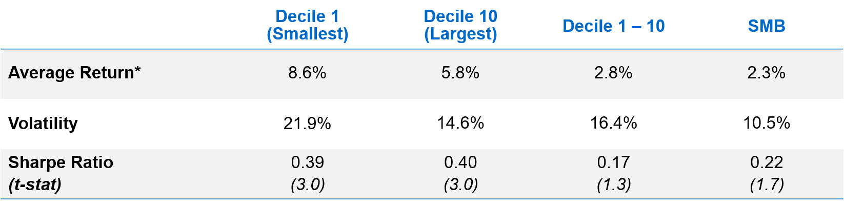
I use the industry standard data from Ken French’s website. I look at the returns to size deciles 1 through 10, the returns on the SMB factor, 8 and market portfolio returns, all for the USA from July 1963 – June 2020 9 (I will also occasionally mention the 1990 – 2020 results just to make sure this isn’t all a problem with the early data – it isn’t).
Let’s start with univariate data (i.e., unadjusted for any factor exposure including market beta).

* All long-only portfolio returns are excess of T-bills and averages are arithmetic.
Source: AQR, Ken French Data Library. Based on monthly returns July 1963 – June 2020. Data description provided in the Ap …
We do see a size premium in the raw returns (though the Decile 1 (smallest) portfolio is volatile enough that it actually has a slightly lower Sharpe than Decile 10 (largest)). Also, even with near 60 years of data you get only an approximately 0.2 Sharpe and a t-statistic well south of 2.0 on the spread between small and large (the two far right columns), which gets you to a very marginally statistically significant result. That is pretty unimpressive even before what are likely large implementation costs. So, the size effect is already in big trouble. I’m going to make it worse. The next table shows that even the simplest, and I’ll soon argue insufficient, beta adjustment cuts away roughly half of small stocks’ average return edge over large stocks.
Table 2 – Monthly Regression on Market Factor

* For the long-only portfolios (deciles 1 and 10) this is a T-test of the market beta vs. 1.0. For the long-short portfolios (Decile 1-10 and SMB) it’s a T-test of the market beta vs. 0.0.
Source: AQR, Ken …
OK, so we haven’t even gotten fancy by introducing the lagged market to adjust for illiquidity, and already there is pretty much no size effect net of the larger betas of small stocks. 10 Now we’re going to dance on the size effect’s grave a bit more.
All I’m going to do now is add one more term to the regression, the market return lagged a month. Again, the idea is if small stocks don’t always trade, they may have fallen (increased) in value in a market drop (rise), but you just can’t pick it up with contemporaneous regressions. Thus, if small stocks also show a positive beta to last month’s market return, it’s very likely because they really did fall (or rise) in value with the market last month even though no price change was recorded because of illiquidity. Adding up the current and lagged beta can give us a better idea of the true beta and thus the true hurdle before we can say there’s positive return excess of beta exposure. So, the next table repeats the above just adding in that lagged monthly market return.
Table 3 – Monthly Regression on Market Factor Plus Lag

* Like earlier for the long-only portfolios (deciles 1 and 10) this is a T-test of the market beta vs. 1.0. For the long-short
portfolios (Decile 1-10 and SMB) it’s a T-test of the market beta vs. 0 …
So, this is a fine mess if you’re a fan of the classic simple size effect (only adjusting for market beta but this time adjusting more accurately by using the contemporaneous and one month lagged market). The alpha of Decile 1 is very mildly negative for ~57 years with a very significant lagged beta of 0.25 (taking the total estimate of beta from an estimated 1.10 to 1.35, which is a non-trivially higher hurdle to overcome given a positive equity risk premium). The 1990-2020 results are even worse for alpha (-1.2% per annum after summed beta adjustment) with its own highly significant lags (so the illiquidity driving the simple regression’s underestimation of market beta is not just an early sample phenomenon).
OK, now let’s look at daily data (yes, I’m finally getting to the actual point!).
Table 4 – Daily Summary Stats

* All long-only portfolio returns are excess of T-bills.
Source: AQR, Ken French Data Library. Based on daily returns July 1, 1963 – June 30, 2020. Data description provided in the Appendix. Hypothetical da …
The summary stats are quite similar but a little off from the annualized monthly summary stats (I suspect it has to do with how the site compounds daily returns). Let’s regress these portfolios on the market now (no lags yet).
Table 5 – Daily Regression on Market Factor

Source: AQR, Ken French Data Library. Based on daily returns July 1, 1963 – June 30, 2020. Data description provided in the Appendix. Hypothetical data has inherent limitations, some of which are described in the …
This (Table 5) is as good as it’s going to get for the small firm effect. Suddenly there is one and it’s actually higher than before we beta-adjusted the daily data. But, note two things:
1) It’s still not that good (alpha t-stats getting close to but not quite reaching 2.0).
2) The table is so misleading I’d call it broken.
How is it misleading? Well, notice first the regression beta of Decile 1 on the market portfolio. It’s 0.74 and a -53.8 t-stat below 1.0. Huh? Isn’t both our intuition and the evidence in many other places (including Tables 2 and 3 above) that small stocks have high betas? But here the smallest portfolio has a beta of 0.74 and both long-short portfolios (Decile 1-10 and SMB) have negative betas, which importantly is what’s driving their newly positive alphas (suddenly their returns look more impressive as if you have a negative beta you expect that to hurt you long-term, and these are the results net of that). What’s going on?
What’s going on is illiquidity. We already argued above, and then illustrated with monthly data, that small firms might not trade so often, and thus regressions of monthly small stock returns on the same monthly market returns might show betas that are biased low (because not trading is a great way to look low beta!). 11 Well, if that effect shows up monthly it just makes sense that it shows up on steroids when measured daily. Measured daily, the smallest firms, which clearly have betas well > 1.0 in all other tests, show up as having betas substantially < 1.0 just by virtue of illiquidity. If that’s the case, then the barely statistically significant alphas in Table 5 are overstated, as beating 74% (the daily beta above of Decile 1) of the market’s excess return over time is a lot easier than beating, say, 120% of the market’s risk premium. Below I regress these same portfolios on the same contemporaneous daily market return as in Table 5 above, but also on the prior day’s market return (lag 1) and the average market return over the nine days before that (lags 2-10). 12
Table 6 – Daily Regression on Market Factor Plus Lags 1 and 2-10

* Like earlier for the long-only portfolios (deciles 1 and 10) this is a T-test of the market beta vs. 1.0. For the long-short portfolios (Decile 1 vs. 10 and SMB) it’s a T-test of the market beta vs. 0.0.
OK, that’s a pretty extreme set of regressions. Look at just long-only Decile 1. Its beta on the market’s move the same day is the same as the univariate regression in Table 5, 0.74. But its beta to the day before that is 0.12, and to the move over the prior nine days it’s 0.33, both highly statistically significant. Thus, the total estimate of beta is 1.19. That’s a lot bigger of a hurdle than 0.74 alone and turns the alpha from 2.3% per annum in Table 5 to -0.6% here. For the difference between deciles 1 and 10, the contemporaneous beta of -0.27 (again, that screams wrong as it says the beta of the smallest firms is lower than that of the largest) is actually too low by a whopping 0.55 (0.16 + 0.39 from the table), meaning our estimate of the real beta is not -0.27 but instead 0.28. That changes the apparent excess of market return of decile 1 vs. 10 from a reported (but fictitious) 2.8% per annum in Table 5 to what we think is a more accurate -0.8% here.
Again, admittedly, the daily results don’t show anything that leads to different conclusions than the monthly results. But I think they show what’s going on considerably more starkly. In the monthly case, the betas of small stocks are greater than large ones even measured using simple contemporaneous regressions, but illiquidity causes us to underestimate how much larger. In the daily case, the betas of small stocks actually come out much (economically and statistically) smaller than those of large ones if we don’t adjust for illiquidity. When we do adjust for illiquidity (with the lags), sanity is restored.
To summarize,
- Small stocks beat large stocks historically but that’s only before adjusting for market beta, an adjustment we’ve all been doing in this field when studying size since the early 1980s.
- Any way you slice the above there is nothing even resembling a long-term simple small firm effect (where the returns of small stocks are greater than larger ones by more than implied by their market betas).
- Adding in lags to account for illiquidity takes the historically weak small firm effect and renders it non-existent.
- This is most clear when looking at daily returns. Small stocks are so illiquid that even though they truly have betas considerably greater than large stocks, simple contemporaneous regressions erroneously show them to be much smaller. Adjusting for that leads to a dramatic turnaround in beta (and dramatic reduction in realized alpha) that perhaps even better illustrates the phenomenon than the monthly results we’ve focused on in prior work.
- In separate work we show a different size effect, the size effect net of the quality factor, is quite strong (though we acknowledge this finding is not obviously implementable). This is not at all inconsistent with the results here.
- Finally, as we have said before, whether other anomalies (e.g., value, momentum, etc.) work better among small firms is by itself interesting, and this can also render something like “small value” a long-term attractive strategy.
So, if you had doubts, maybe now the size effect really is “settled”!
Appendix
Data Description
All data is based off monthly and daily returns from the Kenneth R. French online Data Library (https://www.valuewalk.com/wp-content/uploads/2021/07/clost.pngwww.valuewalk.com/wp-content/uploads/2021/07/clost.pngwww.valuewalk.com/wp-content/uploads/2021/07/clost.pngwww.valuewalk.com/wp-content/uploads/2021/07/clost.pngwww.valuewalk.com/wp-content/uploads/2021/07/clost.pngwww.valuewalk.com/wp-content/uploads/2021/07/clost.pngmba.tuck.dartmouth.edu/pages/faculty/ken.french/data_library.html). The universe is U.S. all-cap that combines the NYSE, AMEX and NASDAQ.
Returns of size deciles (used for Decile 1, Decile 10, and Decile 1-10) are from French’s “Portfolios Formed on Size.”
Returns of the SMB factor and the market (excess of the risk-free rate) are from French’s “Fama/French 3 Factors” and based on Fama and French (1993). The SMB (Small Minus Big) factor is constructed using 6 value-weight portfolios formed on size (small and big) and book-to-market (value, neutral, and growth), taking the average return of the three small portfolios minus the average return of the three big portfolios.
Article by Cliff Asness, AQR