Key Points
- The value premium is traditionally associated with stock selection and market timing, however, value investing works just as well when applied globally across major asset classes.
- The alternative value portfolios we study are typically uncorrelated with their underlying asset classes, traditional value approaches, and each other, thereby offering meaningful diversification benefits alongside attractive excess return potential.
- The success of value portfolios hinges on their design, which allows investors to gain better exposure to desired risk premia not easily available when investing in a single market.
“Buy cheap and sell dear.”- Benjamin Graham, The Intelligent Investor

Check out our H2 hedge fund letters here.
Value investing, a well-known and popular strategy, enjoys broad adoption in the investment community and is supported by a wide array of academic articles. Investors likely associate the word “value” with terms such as book-to-market ratio, price-to-earnings ratio, and bond yield, which are traditionally used for selecting investments in individual stocks, an entire equity market, or local government bonds. A robust body of literature, however, indicates that value strategies work just as well when investing globally across international equity indices, foreign government bonds, currencies, and commodities.1
Global value portfolios are indeed attractive. As we review in this article, these strategies offer notable risk-adjusted returns, which are largely uncorrelated with the underlying markets. Moreover, they have succeeded when traditional value approaches have fallen short. For instance, using valuations to invest across global equity markets and international government bonds has proven to be a worthwhile endeavor. In contrast, equity valuations and bond yields have been of little help in predicting mean reversion within US stock and bond markets (e.g., Masturzo, 2017, and Garg and Mazzoleni, 2017).
With significant potential to enhance an investor’s portfolio, a natural question arises: What makes these global value strategies so effective? To fully harvest value premia in global markets, the use of derivatives and shorting may be necessary. Derivative contracts, however, are merely an instrument and alone do not provide sufficient conditions for success. The success of value portfolios hinges on their design, which allows investors to gain better exposure to desired risk premia not easily available when investing in a single market.
We highlight three explanations for the success of global value strategies. First, long–short portfolios allow investors to hedge movements in the markets that may not be simple to time when investing in a single asset. For instance, equity price-to-earnings ratios have been steadily rising over recent decades, compromising their ability to successfully forecast equity markets. Second, global portfolios are well suited to identify and capture alternative sources of value premia, all while controlling for other factors that may not be desired in the portfolio. Indeed, we document that a traditional approach to timing US Treasury bonds may actually have little to do with the value phenomenon. Lastly, diversification is said to be the only free lunch in finance, and this idea applies to the value factor as well. For example, predicting the path of the US dollar against a basket of other major currencies—a single concentrated bet—is more challenging than forecasting the relative path of multiple currencies in a broad basket of currencies—a diversified set of multiple bets.
In sum, value is a robust phenomenon that can take several different forms and its success on a global stage depends on an economically motivated design. Indeed, as emphasized by Israel, Jiang, and Ross (2017), a number of seemingly small decisions can significantly influence subsequent portfolio performance.
Value in Equities: From Traditional Approaches to Global Portfolios
Today’s possibly best-known application of value investing is in the selection of individual stocks. A value strategy selects securities that trade at a discount, or at a price below intrinsic value, a recommendation that goes back at least to Graham and Dodd (1934). In practical terms, investors should seek companies whose stocks are trading at low prices relative to their earnings and book values. This practitioner advice was later validated in the academic community with the pioneering work of Fama and French (1992), whose high-minus-low (HML) factor has since shaped the academic literature on empirical asset pricing.
Valuation metrics can also be used to time an entire equity market. The literature offers a set of relevant metrics to estimate the market’s fair value, an admittedly challenging exercise. In particular, following the work of Campbell and Shiller (1988), the cyclically adjusted price-to-earnings (CAPE) ratio has become a popular indicator of value (e.g., Arnott, Kalesnik, and Masturzo, 2018). The CAPE ratio compares the current market price to the average of the previous 10 years of earnings expressed in today’s dollars, thereby eliminating seasonal fluctuations and smoothing economic cycles. Arnott, Kalesnik, and Masturzo explored this topic in great detail.
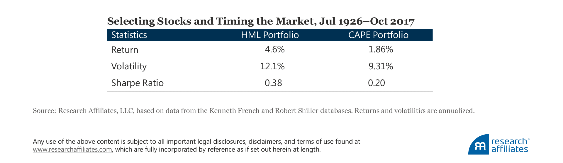
Over the course of the last 90 years, value investing in the United States has proven to be a successful exercise. To appreciate this claim, we summarize the returns of two hypothetical long–short portfolios, which are meant to illustrate the potential excess return earned by traditional value approaches. The first portfolio is the high-minus-low (HML) factor, which is constructed by buying US value stocks—those with a higher book-to-market ratio—and selling US growth stocks; this is done after controlling for companies’ differences in size.2 The second zero-investment portfolio, denominated the CAPE portfolio, tactically allocates between cash and the US stock market using the level of the CAPE as a signal. For instance, when the CAPE ratio is lower than its recent history, the portfolio is bullish and invests in the stock market by borrowing at the cash rate; otherwise, it does the opposite and takes a bearish view.3
The historical evidence in the US market—a 0.38 Sharpe ratio for the HML portfolio and 0.20 for the CAPE portfolio from July 1926 through October 2017, both correlations are statistically significant—suggests that the value premium as traditionally applied is real, and that adjusting portfolio exposures based on these value metrics can lead to outperformance. But Benjamin Graham’s time-tested advice to “buy cheap and sell dear” does not need to be limited to single securities or markets. If buying below and selling above intrinsic value has proven effective both within the equity market and at the equity market level, we might naturally expect a value-oriented approach to prove fruitful when applied across the world’s equity markets.
By drawing a parallel between individual stocks and markets, we next build an HML strategy applied to 12 developed country equity markets. This alternative value strategy takes equally weighted long positions in the top-third most attractively valued equity markets and equally weighted short positions in the bottom-third least attractively valued equity markets across the developed world. We use market indices and local cash rates to compute each of the 12 markets’ excess return, and the portfolio is rebalanced monthly.4
Similar to individual stock analysis, we rank equity markets by their book-to-market ratio. Markets with a high book-to-market ratio are deemed cheap, and markets with a low ratio are deemed expensive. We call this strategy the Global portfolio, and it has indeed proven successful over about 30 years (March 1985 through October 2017). This long–short portfolio logged a Sharpe ratio of 0.42, a remarkable source of excess return having the added benefit of being largely uncorrelated with both of the more-traditional HML and CAPE portfolios, and the US stock market.

In contrast to the HML and CAPE strategies, the Global portfolio has not disappointed over the most-recent 30-year sample period. The premium offered by the HML strategy, for example, has almost been halved with respect to the full-sample evidence (2.7% versus 4.6%), and the premium offered by the CAPE strategy has been null (−0.2%). What happened to these two traditional value portfolios? And where is the resilience of this alternative Global portfolio coming from?
A correlation matrix sheds some light on the dynamics of these three portfolios. The global approach displays, on average, a null association with the other two value portfolios, whereas the 0.31 correlation between the HML and CAPE strategies over the period is positive and quantitatively significant. As pointed out by Israel and Ross (2017), the latter pattern is explained by the significant market bets that a simple implementation of the HML factor has taken over the years. In short, despite being a long–short portfolio, the HML portfolio has, on average, been short equity beta along with the CAPE portfolio.
The resilience of the Global portfolio is primarily due to its design: being simultaneously long and short allows the strategy to hedge the common global equity premium shared by developed equity markets. International equity markets display a high degree of co-movement, and this common variation has been difficult to time. Specifically, equity markets have appreciated over the last few decades according to various valuation metrics, and this continuous upward trend explains the underperformance of the CAPE portfolio, which has largely had a short position in the US stock market.5
To illustrate the importance of the Global portfolio’s design, let’s consider a simple twist to its construction. This time, we rank each country based on the level of its book-to-market ratio with respect to its trailing historical average, and then buy any country that is accordingly deemed expensive or sell it otherwise. (We ignore any cross-sectional information and exclusively rely on time-series information.) This new portfolio performs very similarly to the CAPE portfolio, offering an insignificant excess return. Further, its correlation with the CAPE portfolio jumps to approximately 0.60, despite its being diversified across 12 developed equity markets. In other words, this twist in design led to significantly negative market exposure—not a desirable outcome.
Inspired by the attractive characteristics of the global equity strategy, we next explore an alternative value approach across global government bonds.
Value in Bonds: From the Term Spread to Real Yields
As with equities, a natural definition of value in government bonds would likely rely on some price-to-fundamental ratio. Government bonds are expected to pay a coupon (interest) and repay principal, which conveniently allow investors to compute a bond’s yield. Combinations of bond yields can be very useful predictors of bond excess returns (e.g., Cochrane and Piazzesi, 2005). Yet, there’s a catch: a successful predictor of bond returns may be forecasting multiple sources of risk premia and not just mean reversion in prices.
To understand value in government bonds, let’s start by focusing on the 10-year US Treasury bond and two metrics suggested by Asness, Moskowitz, and Pedersen (2013) in their international study: the term spread and the 10-year real yield. In our study, we define the term spread—likely the best-known predictor of bond returns—as the difference between the yields of the 10-year US Treasury bond and the 3-month US Treasury bill. We define the 10-year real yield as the current nominal yield minus the trailing five-year average core inflation rate. These two measures can be understood as different ways to measure a bond’s valuation.
We assess these valuation metrics by constructing two tactical portfolios. The first portfolio, which we call the term-spread portfolio, invests in the 10-year bond by borrowing at the cash rate if the spread is above its trailing average level. Otherwise, it shorts the bond and invests in cash. The second portfolio, which we call the real-yield portfolio, follows a similar strategy, but uses the level of the 10-year real yield relative to its trailing average level as the value indicator.
Our results clearly illustrate why the term spread is a very popular predictor of returns, whereas the real yield alone never makes the headlines. The overall performance of the two portfolios—represented by their respective annualized total returns (3.4% for the term-spread portfolio versus −0.7% for the real-yield portfolio)—is quite different. The term portfolio offers a notable 0.47 Sharpe ratio, whereas the Sharpe ratio of the strategy based on the relative level of the real yield is null. A comparison of the total returns, however, may lead to a premature conclusion.
To fully appreciate the value added by the term-spread portfolio, we can decompose the two portfolios’ returns into spot and carry components. As emphasized by Koijen et al. (2016), carry is a significant component of many successful strategies, and it corresponds to the returns that would be realized if spot prices did not change; that is, the difference between the total return and carry is explained by price movements in the cash market:
Total Return = Carry Return + Spot Return
Therefore, the difference between the total return and the spot return is simply the carry tilt of a portfolio. This decomposition teaches us two things: first, a bit less than half of the term-spread portfolio’s return (3.4% − 2.0% = 1.4%) is due to the carry factor, not to mean reversion in valuations; and second, the real-yield portfolio takes consistent negative carry bets, which wash away any potential excess return.
Although we do not show it here, a look at the correlation (0.44) of the return of the term-spread portfolio with the return of a simple long-bond position further reveals the nature of the term-spread signal. Because of falling yields over the March 1989–October 2017 period, the term-spread portfolio has had a net positive bond market exposure, which entirely explains the spot component of its return. All in all, the term-spread signal did not display any obvious value tilt in our out-of-sample exercise applied to the US Treasury market.
Once again, a persistent fall in bond yields since the early 1980s greatly complicates the life of a US contrarian investor, whether she uses the term spread or the real yield as an investment signal. And just like for the equity analysis, a valid alternative is offered by a global approach to value investing.
To assess the validity of a global approach to value investing across government bonds, we create two global bond portfolios. The global term-spread portfolio’s positions are driven by a cross-sectional comparison of the term spread, and the global real-yield portfolio’s positions are determined by a cross-sectional comparison of the 10-year real yield. By using a sample of eight developed, liquid markets, these strategies take equally weighted long positions in the top-third group of countries with the highest signal and equally weighted short positions in the bottom-third with the lowest signals. We estimate government bond futures’ returns and the portfolios are rebalanced monthly.6
The global evidence is clear. By relying on cross-sectional information, the real-yield portfolio offers a positive excess return, all of which is in the form of spot price movements (spot return of 0.7% versus total return of 0.5%). In addition, the correlation between the returns of the global portfolio and its original US version is positive (0.26), further lending support to its economic rationale. Instead, the correlation with the return of the global term-spread portfolio is negative (−0.33), indicating the difference in nature between these two strategies.
Clearly, the real-yield signal offers the most relevant metric to gauge value for bond investors, whereas the term-spread portfolio is best utilized as a carry strategy, a worthwhile topic, but one that lies outside the scope of this article.
Additional Sources of Value: Currency and Commodity Approaches
Two other assets tend to make the headlines of financial newspapers: the US dollar and the price of oil futures. As such, investors may be tempted to try to time these two assets based on their perceived valuations. But as has been the case with equities and bonds, market timing can be a tricky exercise, and the US dollar and oil are no exceptions. In particular, neither the US dollar nor oil pays a dividend, which greatly complicates the search for a convincing valuation metric. Hence, we conclude our empirical analysis by offering a simple solution: diversify your bets!7
To appreciate the benefits of diversification, we constructed our usual 1/3 long and 1/3 short portfolios applied across 10 developed currencies and 24 commodities.8 Because these assets do not pay a dividend, we chose to adhere to the literature to gauge their valuations through the five-year change in their real price (e.g., Asness, Moskowitz, and Pedersen 2013). To put it simply, over the periods we analyzed, the currency and commodity asset classes are no exception to the evidence supporting the existence of a value premium (0.40 and 0.31 Sharpe ratios, respectively), and both portfolios offer excess returns uncorrelated with the underlying asset class.
Notably, the Currency portfolio is still closely related to the dynamics of the US dollar. We find that when the dollar mean reverts to fair value, so do all of the other currencies, which is suggestive of a time-varying exposure of the Currency portfolio to the average dollar returns. The key finding of our analysis is that the best approach is to invest in the potential mean reversion of several currencies rather than just one.
The excess returns generated by the alternative value portfolios we’ve introduced in this article are uncorrelated with traditional asset classes and value approaches, and they are lightly correlated with each other, with an average cross correlation of about 0.13. In particular, a mild association exists between the bond portfolio and its equity and currency counterparts, which is suggestive of the global nature of the value phenomenon and its sound economic foundation.
Conclusion
In this article, we have reviewed the evidence and rationale in favor of the global dimensions of value investing. By comparing and contrasting traditional value trades with their global alternatives, we have highlighted the latter’s ability to harvest uncorrelated sources of risk premia, an essential source of return available to investors seeking to improve their performance prospects.
Given these beneficial properties, an investor may naturally ask: Are global value portfolios too good to be true? We argue that their past strength and future success rely significantly on an economically motivated design. In particular, by studying equity market indices, international government bonds, foreign currencies, and commodities, we highlight three features that help explain the positive performance of such strategies. First, a long–short portfolio allows investors to shield themselves from movements in market direction that may be difficult to time. Second, global portfolios are well suited to identify and isolate alternative sources of value premia and hedge away other drivers of returns, which may not be desired in the portfolio. Lastly, diversification is the closest thing in finance to a free lunch, and this concept obviously extends to value investing in its many forms. In short, when value goes global, investors are poised to benefit.
Article by Brandon Kunz, Michele Mazzoleni - Research Affiliates