Hoisington Investment Management Company commentary for the fourth quarter ended December 31, 2017.

Optimism is pervasive regarding U.S. economic growth in 2018. Based on the solid 3%+ growth rate during the last three quarters of 2017, this optimism is well-founded. The acknowledgement of this economic health by the Federal Reserve (Fed) is evident: they have outlined a continued pattern of increasing the federal funds rate over the coming year. Further, the solid 2017 performance of the European Union and of Japan is forecast to continue in 2018. Finally, the recent enactment of a tax cut is expected to boost U.S. economic growth in the new year. Well-regarded economic research suggests a 2.5% - 3.5% real growth rate in 2018 with continuing stable inflation. In addition, most surveys suggest a modest interest rate increase across the entire maturity spectrum of the yield curve.
Our view of the economic environment is somewhat divergent from the consensus opinion. Our analysis of concurrent and leading economic variables, including consumers, taxes, monetary policy and the yield curve, suggest that disappointing growth, lower inflation and ultimately lower long-term interest rates will hallmark the new year.
Consumers
Consumer spending, the economic heavy lifter of U.S. economic growth, has expanded by 2.7% over the past year (as measured by real personal consumption expenditures, or PCE, as of November 2017). This is similar to the past eight years of the expansion, with real PCE averaging 2.5%. What is interesting about the increase in spending is that incomes have failed to keep pace. Real disposable personal income rose by only 1.9% over the past year. It was only the ability to borrow that supported the spending increase. In economic terms, borrowing is a form of dissaving. The saving rate for consumers dropped from 3.7% a year ago to 2.9% in November, a 10-year low.
It is remarkable that as recently as October 2015 the consumer saving rate was 5.9%. Had that rate been sustained through November 2017, the cumulative spending increase over the past 25 months would have registered only a 3.2% advance (1.5% annual rate) or $496 billion. However, actual spending was $939 billion, a 7.5% cumulative gain (2.8% annual rate). An increase in consumer credit of $253 billion and an actual reduction in savings of $190 billion account for this difference. It is possible that the saving rate will continue to fall. A drop of the same magnitude in the next 25 months would mean the saving rate would be -0.1%, a possible yet unlikely scenario. The higher probability is that the saving rate begins to move up towards its historic average of 8.5%.
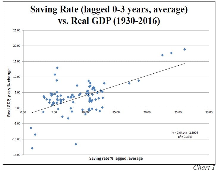
History suggests that the economy will register a slower rate of expansion following a low saving rate (Chart 1). This positive correlation between current saving and future consumption means a low saving rate should be followed by a lower level of consumption and vice versa. Therefore, considering that the only period in which the saving rate was lower than it is today was 1929–1931, it is more likely that spending in the future will be in line with, or lower than, real income growth, which is currently weak.
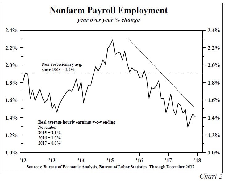
Furthermore, the modest increase in real disposable income of 1.9% over the past twelve months will be under downward pressure in 2018 as employment growth continues to slow. Employment growth actually peaked in early 2015, expanding year-over-year by 2.3%. However, by December 2017 the growth rate had diminished to 1.4% (Chart 2). This slowing trend will persist in 2018, placing downward pressure on income gains and therefore on spending as well.
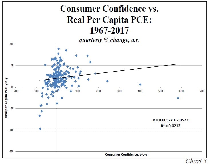
Conventional wisdom suggests that rising consumer confidence significantly boosts spending. However, plotting the quarterly percent changes in real per capita PCE against percent changes in consumer confidence from 1967 through the third quarter 2017, it appears that consumer confidence is unreliably related to real PCE (Chart 3). Over this very robust sample of 202 observations, a 1% gain in confidence only boosts real per capita PCE by a minuscule 0.006%. While the correlation is positive, the relationship is not statistically significant with a coefficient of determination (R2) of only 0.02.
Finally, borrowing should slow in 2018. The 125 basis point increase in the federal funds rate since December 2015, and its magnified effect on short-term financing rates, coupled with deteriorating loan quality, should continue to reinforce the slow-down in borrowing at the consumer level. Therefore, both the supply and demand for credit is waning. Slower borrowing and modest income expansion, along with a potential reversal in the near historic low saving rate, means consumer spending will likely be one area of economic disappointment in 2018.
Taxes
In 1820, the great economist David Ricardo (1772-1823) was asked whether it made any difference to the overall British economy if the Napoleonic Wars were financed by an increase in debt or by an increase in taxes. He theorized that the two were equivalent (the Ricardian Equivalence). However, Ricardo candidly cautioned that his theory might not be valid. Indeed, continuous streams of data and statistical computing techniques t Sources: Bureau of Economic Analysis, Bureau of Labor Statistics. Through December 2017. hat are available today were not available in the early 1800s to test his theory.
The economics profession followed Ricardo’s theory until 1936 when John Maynard Keynes (1883-1946) introduced the government multiplier concept. It posited that $1.00 of debt financing would expand GDP by some multiple of that amount. Keynes, like Ricardo, did not offer empirical proof for his proposition. And like Ricardo, it is doubtful he could have produced such analysis given the lack of advanced statistical computing techniques at that time.
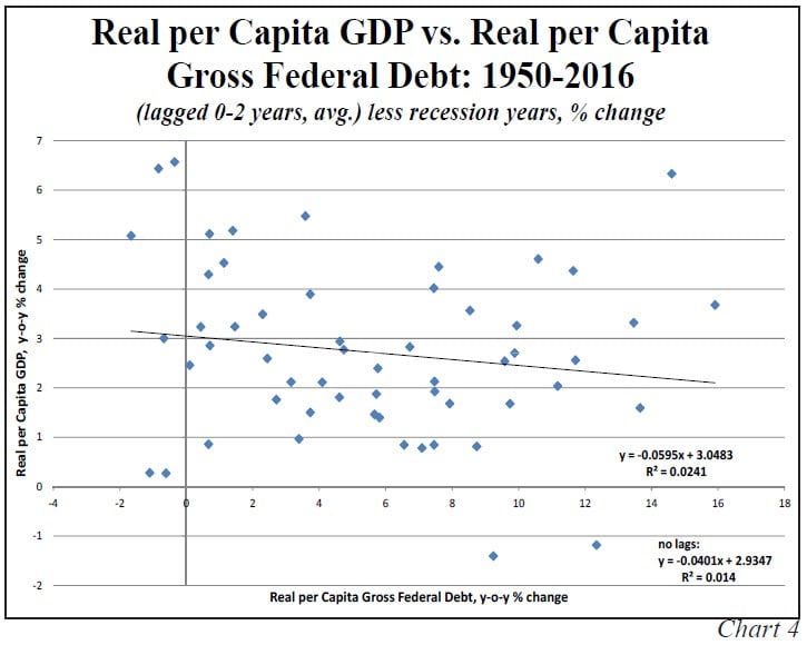
To further analyze these theories, using data from 1950 through 2016, we developed a scatter diagram plotting the year-over-year percent change in real per capita GDP against real per capita gross federal debt, with lags in the debt of one and two years, equally weighting each year (Chart 4). We added the prior two years in order to capture any lags in the response of the economy to the debt changes. The results of this diagram add to the evidence that Ricardo’s theory was correct. The most important conclusion of this extensive data set, which excludes recessions, is that the slope of the line is negative but not statistically significant. A 1% increase in debt per capita over three years results in a slight decline in real per capita GDP of 0.06%, and the coefficient of determination (R2) is just 0.02. If the scatter diagram is calculated without lags, the slope is a virtually identical -0.04, with an even lesser R2 of 0.01. In short, these results align with Ricardo’s theory; although individual winners and losers may arise, a debt-financed tax cut will provide no net aggregate benefit to the macro-economy.
If the tax cuts were instead to be financed by a reduction in expenditures (revenue-neutral), then the economic growth rate would benefit to a minor degree. Since productivity is higher in the private sector than in the government sector, tax cuts should have a more favorable multiplier. In this type of revenue-neutral package, the economy would thus receive a slight boost. The tax cuts should increase incentives and efficiencies, and possibly lower the cost of capital and moderate the increase in the steady and substantial rise in federal debt.
Federal debt, however, still remains a problem since gross government debt recently exceeded 106% of GDP. A debt level above 90% has been shown to diminish an economy’s trend rate of growth by one-third or more. When President Reagan cut taxes in 1981 growth ensued, but the government debt was only 31% of GDP, an economic millennium from our present 106%. Looking forward, the Joint Committee on Taxation expects a $451 billion revenue gain from improved growth over the next ten years, yet it still expects the recent tax bill to add $1.1 trillion to the deficit. The Congressional Budget Office expects a $1.5 trillion increase in the deficit over the same period. According to some private forecasters, due to the front-loading of some provisions, for the next two years the federal deficit will be rising – moving from roughly 3.6% of GDP in fiscal 2017 to 3.7% of GDP in fiscal 2018 to 5% of GDP in 2019. Thus, the continuing debt buildup will have the unintended consequence of slowing economic growth in 2018 and beyond, despite the favorable multiplier contribution that individual tax cuts impart.
Monetary Policy
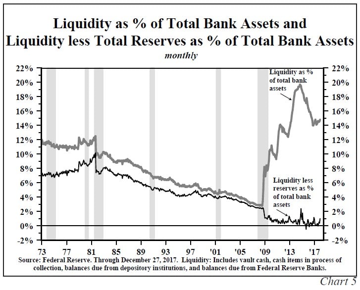
Although the economy may slow due to a poor consumer spending outlook and increases in debt, the real roadblock for economic acceleration in 2018 is past, present and possibly future monetary policy actions. The Fed first began raising the federal funds rate in December 2015. A year later the Fed implemented another 25 basis point increase. Three more rate hikes occurred in 2017. To raise interest rates the Fed takes actions that reduce the liquidity of the banking system (Chart 5). This action has historically caused a reduction in the supply of credit through tighter bank lending standards. The demand for credit is also diminished as some borrowers are priced out of the market or can no longer meet the higher quality standards.
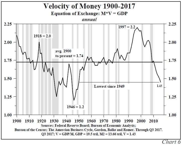
The impact of this tightened Fed policy on money, credit and eventually economic growth is slow but inexorable. The brunt of these past and current policy moves will be felt in 2018. Irving Fisher provided the arithmetic formula that money times its turnover equals price times transactions, or nominal GDP (MV=PT). This simple equation provides a roadmap of ebbing growth next year. Velocity (V) is currently low. At 1.43, velocity is standing at its lowest level since 1949, well below the 1.74 average since 1900 (Chart 6). Money (as defined by M2) expanded by 7% in 2016. Owing to Fed actions, money growth slowed to a 5% year-over-year growth rate at the end of the third quarter 2017, a 2.5% reduction from the previous year. In the fourth quarter of 2017 the Fed planned to reduce its balance sheet by $30 billion, an action we term “quantitative tightening” (QT). This action has and will continue to put additional downward pressure on money growth; a $60 billion reduction is expected in the first quarter of 2018, a $90 billion reduction is expected in the second quarter of 2018, and an additional $270 billion in reductions are expected following the second quarter of 2018. It is important to note that historical comparisons and analysis are unavailable as the magnitude of this balance sheet reduction is unprecedented; however, the threemonth growth rate of money has already slowed further to 3.9% at the end of 2017.
In the 1960s, economists Karl Brunner (1916-1989) and Allan Meltzer (1928-2017) both proved M2 equals the monetary base (MB) times the money multiplier (m) (M2=MB*m). They also algebraically identified the determinants of m. Application of their model, which has been verified by numerous others, suggests the monetary slowdown will intensify, thereby increasing the drag on economic growth, as 2018 unfolds. If the Fed continues QT for one year as outlined, we calculate the overall change in M2 could turn negative by the end of the year. If money (M2) continues to decelerate, and V stabilizes (although it has declined at a 2.4% rate over the past eight years), then nominal GDP will record a lower growth rate in 2018 than the estimated 2017 pace of 4.0%.
Yield Curve
The determinants of short-term interest rates are far different than those of long-term interest rates, thus causing the shape of the Treasury yield curve to significantly change shape over the course of the business cycle.
Changes in long-term Treasury bond yields are determined by the Fisher equation, one of the pillars of macroeconomics. In this equation, the nominal risk-free bond yield equals the real yield plus expected inflation (i=r+πe). Expected inflation may be slow to adjust to reality, but the historical record indicates that the adjustment inevitably occurs. Although very volatile over the short-run, the real rate can be stable over longer time spans; inflationary expectations ultimately dominate the longer run movements in the Treasury bond yield. The Fisher equation can be rearranged algebraically so that the real yield is equal to the nominal yield minus expected inflation (r=i–πe).
Short-term interest rates are determined by the intersection of the demand and supply of credit that the Fed largely controls through shifting the monetary base and interest rates. The higher funds rate can be reached by a slower but still positive growth rate in the monetary base or by an outright decline in the base. When the base money becomes less available, the upward sloping credit supply curve shifts inward, thus hitting the downward sloping credit demand curve at a higher interest rate level.
Restrictive monetary policy impacts the economy through several observable phases, all of which take time to work. Initially, the monetary shift causes the federal funds rate to rise. As mentioned earlier, as the federal funds rate moves higher, the growth rates of the monetary and credit aggregates slow. A sign that this restrictive process is beginning to more meaningfully impact monetary conditions is that the yield curve begins to flatten, with short-term rates rising relative to long-term rates. Historically, as the yield curve flattens, the profitability of the banks and all similarly structured entities is diminished from this influence. Thus, initially the change in the curve is a symptom of monetary tightness, but the flatter curve reinforces the earlier monetary restraint.
Outlook
The full spectrum of monetary policy is aligned against stronger growth in 2018. A higher federal funds rate, the continuation of QT, low velocity and abruptly slowing money growth all put downward pressure on growth. The flatter yield curve will further tighten monetary conditions. This monetary environment coupled with a heavily indebted economy, a low-saving consumer and well-known existing conditions of poor demographics suggest 2018 will bring economic disappointments. Inflation will subside along with growth causing lower long-term Treasury yields.
Van R. Hoisington
Lacy H. Hunt, Ph.D.
Performance
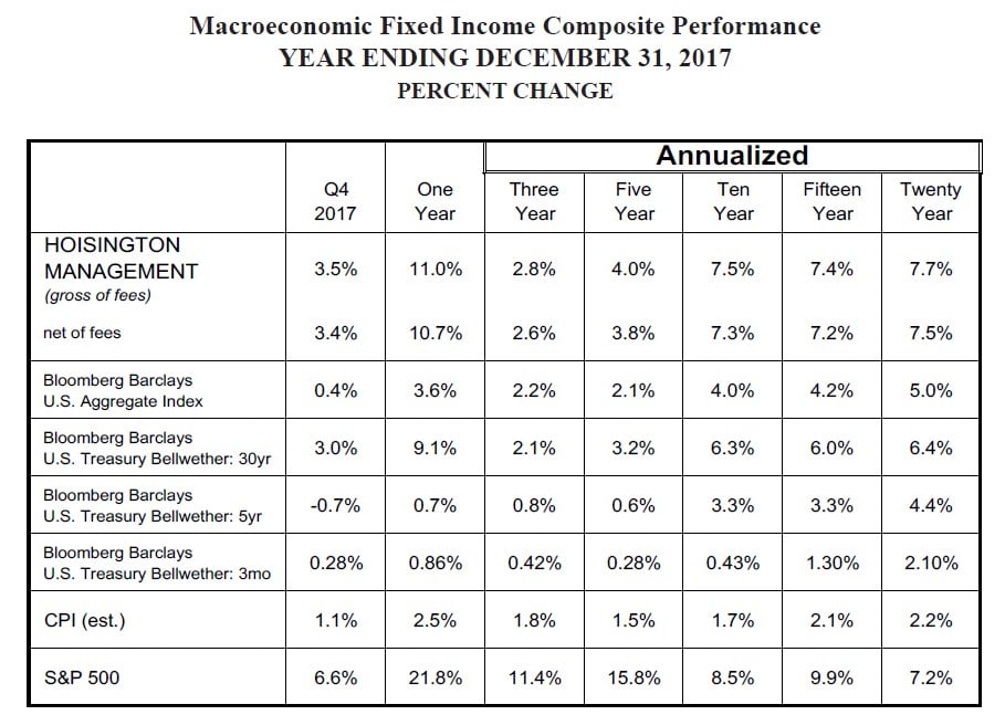
HIMCO’s Macroeconomic Fixed Income Composite, which is invested in U.S. Treasury securities, registered a net return of 3.4% for the fourth quarter of 2017 and 10.7% for the year. The Bloomberg Barclays U.S. Aggregate Index had a return of 0.4% for the quarter and 3.6% for the year. In an unusual event, 2017 witnessed the rise in short-term interest rates while long-term interest rates declined. For instance, the two-year Treasury Note went up in yield by about 70 basis points while the 30-year Treasury Bond declined by about 33 basis points. This explains the wide gap in performance between the index and the HIMCO composite. For the past three, five, ten, fifteen and twenty year annualized periods HIMCO’s composite net returns outperformed the index by 0.4%, 1.7%, 3.3%, 3.0% and 2.5%, respectively.
See the full PDF below.


