Executive summary
- Recognizing that markets are a “Loser’s Game” means minimizing mistakes should be a more successful strategy than attempting to select winners
- Equity “Smart Beta” factors are mostly priced into markets and therefore should offer little opportunity for outperformance
- Value and Momentum metrics appear more successful at selecting securities compared to other smart beta factors
- Quality, Volatility, and Price Reversal metrics tend to be priced into markets but at their extremes may be useful for avoiding potential poor performers, which concurs with a Loser’s Game
- Many smart beta factors overlap with each other in screening out the most speculative stocks

Q1 hedge fund letters, conference, scoops etc
Introduction
“It is remarkable how much long-term advantage people like us have gotten by trying to be consistently not stupid, instead of trying to be very intelligent.” - Charlie Munger
The right strategy for winning any game requires first understanding the competitive dynamics of the game. One model is that of a “Winner’s Game” versus a “Loser’s Game”. A winner’s game is one where the outcome is determined by the actions of the winner. The most common example used is professional tennis where the winner is usually the one who hits the most winning shots. In contrast a loser’s game is one where the outcome is determined more so by the actions of the loser. Again, in tennis, the amateur game is one where the winner is often the one who commits the fewest unforced errors. In a 1975 paper in the Financial Analysts Journal, Charlie Ellis called investment management a loser’s game1. Professional money managers compete with one another using similar data and analytical models. There is no easy money to be made as these professionals keep markets efficient enough. As a result, the best investors tend to be the ones who make the fewest mistakes, not necessarily the ones who hit the most homeruns. In a Loser’s Game, the right strategy is to avoid making mistakes, rather than trying to score (identify) the big winners.
Markets are efficient enough, most of the time, is another way to sum up the loser’s game. At the very least, making this assumption as our starting point, saves us a lot of pain from poor selection. In contrast, so called “smart” beta strategies, such as high dividend yield or low valuation equity strategies, claim the ability to outperform market averages by screening based on simple quantitative metrics. We think the loser’s game market dynamic is at odds with this claim.
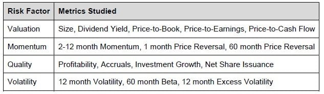
Our research for this paper shows that smart beta factors are mostly priced into markets, but have some utility as a screen to avoid poor performers. We studied 15 quantitative metrics, grouped into four broad buckets of Value, Quality, Momentum and Volatility based measures. While there are claims to the existence of hundreds of risk factors, a growing body of research shows that most are spurious results of data mining or overlap with the four broad risk factors we have used. All of our data is from the Ken French Data Library and each metric we studied had at least 52 years of monthly data with some having over 90 years and going back as far as July 1926. The table below summarizes the metrics we studied and how we grouped them by bucket. Note that while the size factor should be its own unique category, we grouped it with valuation factors for convenience and because value metrics do exhibit some size bias.
We analyze each group of factors for whether they demonstrate any ability to differentiate between high returning and low returning equities, in essence whether the factor is priced into markets.
Value Beats Growth, And Value Historically Provided a Tailwind to Smallcap
Quantitative methods for stock selection have been around for decades. As early as 1976, the father of value investing, Ben Graham, published a formula for selecting cheap stocks that should outperform2. The most commonly used valuation metrics for quantitative models are price-to-book, price-to-earnings, and price-to-cash flow ratios. Lower ratios are meant to signal cheaper prices and therefore higher future returns. However, if we start from a perspective of market efficiency, lower valuation ratios should only imply lower expected growth rates (in sales, earnings, cash flows, etc.) rather than mispriced securities offering higher expected returns.
In reality, there has been a demonstrable bias for lower valuation stocks to outperform those with higher valuations. Some of this bias is likely driven by behavioral factors, such as the propensity to gamble and buy lottery tickets (like a high flying, small cap growth stock), which would drive, on average, overvaluation of speculative stocks. As is only natural in a competitive, capitalist economy, the growth rates of these high flyers tend to revert toward the mean, resulting in falling valuation ratios and lower returns. Since behavioral biases tend to be permanent due to human nature, it is reasonable to expect this lottery ticket anomaly to persist.
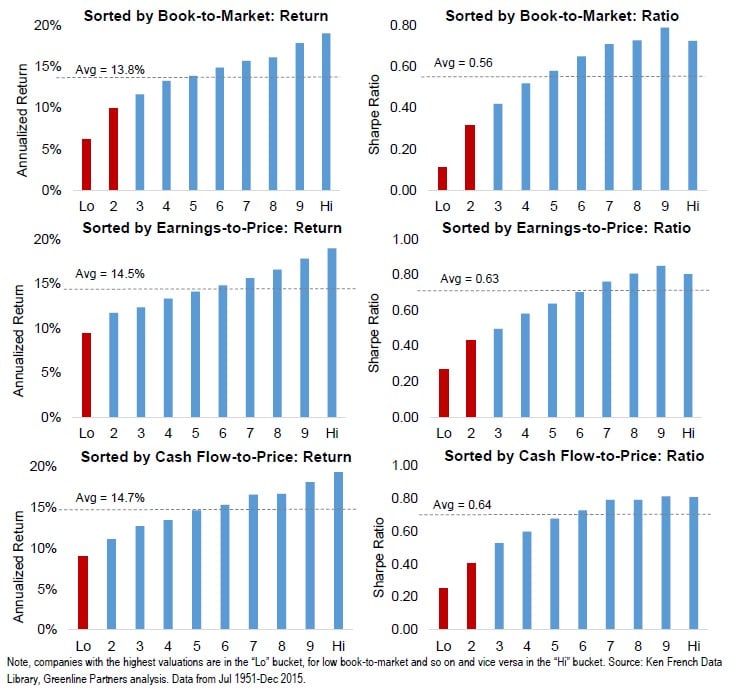
In our study on valuation metrics, we divided the universe of US stocks (using a set similar to the Russell 3000) into 10 equal-weighted buckets, ranked from most expensive to cheapest for each valuation ratio. Each metric studied is the inverse of a traditional valuation ratio, that is we sorted the universe by book-to-market instead of P/B and similarly for P/E and P/CF. Companies with the highest valuations are in the “Lo” or first bucket and the lowest valuation ratios in the “Hi” or tenth bucket.
The charts below on the left side of the page show returns, while those on the right side show the Sharpe ratio for each valuation measure and are based on underlying data from 1951-2015. From looking only at returns, it would appear that these simple valuation measures are not priced into the market and show consistent improvement as one goes from the most “expensive” to “cheapest” buckets, left to right. But risk-adjusted return, as measured by Sharpe ratio, tells a different story. From the charts showing this ratio, we can see a leveling off in the benefit from selecting ”cheaper” stocks. Said another way, there appears to be a greater benefit from avoiding highest valuation equities than selecting those with the lowest valuation. We specifically highlight in red the buckets where the returns and ratios deviate materially from the average. These are all the highest valuation buckets. Each valuation ratio shows the same pattern, that they are more effective at avoiding poor performers than selecting top performers.
We think it is logical that high valuations tend to overestimate future growth, more so than low valuations underestimate growth. When companies and industries grow at fast rates markets tend to expect this growth to continue for many years to come and valuations rise accordingly. The rapid growth attracts competition and capital as is natural in capitalism. Competition not only slows growth but also erodes profit margins dramatically reducing earnings growth. As markets price in this competitive dynamic, usually after growth rates slow, valuations fall, resulting in low returns. Technology companies in the late 1990’s are a prime example of extremely high valuations leading to low returns after competition eroded their potential given the few, low barriers to entry for most. Some businesses undoubtedly achieve rapid growth over long periods of time and deliver on high expectations, but the losses from investing in those who fail to achieve this expected growth are large.
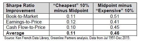
We quantify the advantage of eliminating the worst performers compared to selecting the top performers below. The table compares the improvement in Sharpe ratio from selecting the “cheapest” 10% of stocks compared to the average against the improvement from avoiding the 10% most “expensive” stocks. We can see that the improvement in performance from eliminating the worst has been over 4 times as great as from selecting the best. In technical terms, the benefits from selecting the cheapest equities is not statistically significant, while avoiding the most expensive is.
We generally avoid relying on volatility and Sharpe ratio as measures of risk and risk-adjusted returns because they are not measures of true risk and are easily gamed. But in this case comparing Sharpe ratios across valuation buckets illustrates the concept behind risk-adjusted returns and how the gains from moving to lower valuations are less than linear.
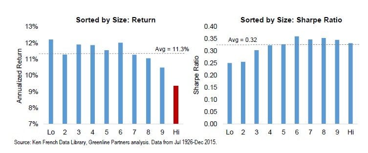
In the above charts, as we move from left to right, absolute returns rise. But by the midpoint of each one, the Sharpe ratios are leveling off indicating that volatility of the underlying stocks is also increasing. There are many reasons why a stock will have higher volatility than others - smaller size and therefore lower earnings stability is one of those reasons. Numerous studies have documented the small cap tilt in value biased investment strategies. To understand the impact of smaller size, similar to the valuation charts above, we sort the market into 10 size buckets. The smallest bucket has an average market capitalization today of ~$100mln (microcap), the middle bucket is ~$2.5bln (smallcap), and the largest averages ~$80bln (mega cap). From the return chart we can see all size buckets earned similar returns historically with a small decrease for large caps (bucket 9) and an almost 2% return reduction for the largest bucket where most investors concentrate their holdings. In the Sharpe ratio chart we see the opposite pattern, that size is largely priced in and each bucket delivers a similar ratio except for the smallest microcap buckets (1 & 2), which have historically earned lower risk-adjusted returns.
The 2% additional return from smaller companies is likely driving part of the return premium from lower valuation equities above. It is logical that lower valuations have a bias toward smaller sizes. If I take two companies with the same sales and earnings, and one has a lower P/E ratio, it will have a smaller market capitalization. This does not explain all of the return improvement from selecting low valuation stocks but a significant part of it.
While academic studies point to the smallcap bias in value investing, we flip the question and ask whether the smallcap return premium was driven by their historically lower valuations. We think the valuation difference was an important driver suggesting there is not a small cap premium. In the 1970’s when smallcap investing was first introduced, this segment of the market had few investors as the companies were considered speculative and had less research coverage and available data. Today, it would be rare to find an institution or individual investor without an allocation to smallcap equities and there are thousands of hedge funds scouring for the those that might outperform. As any information asymmetry was reduced, the smallcap return premium disappeared. Since 1980, smallcaps have actually underperformed largecaps by almost 2% annually3. Today valuations on smallcaps are higher than on the largest companies4 which could lead to lower returns compared to largecaps in the future as well.
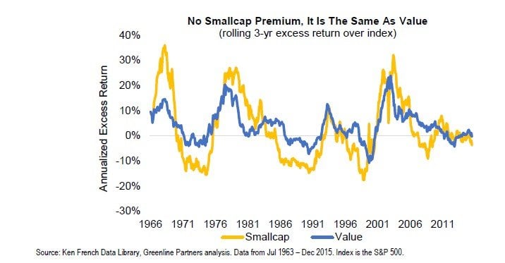
Since there was historically an overlap between low valuation equities and smallcaps we should expect these two styles to have outperformed and underperformed the broad index at the same time. The chart below shows the rolling 3-year excess return of the 2 lowest valuation buckets (low quintile), as defined by earnings-to-price, compared to the excess return of the 2 smallest size buckets (smallest quintile). We can see they both outperform and underperform the broad market at the same time indicating a similar bias. Note that low valuation has lower downside risk and has earned higher absolute returns.
Article by Maneesh Shanbhag, CFA, Chief Investment Officer - Greenline Partners
See the full PDF below.


