by J. L. Kelly, Jr in 1956.[1] The practical use of the formula has been demonstrated.[2][3][4]
Although the Kelly strategy’s promise of doing better than any other strategy seems compelling, some economists have argued strenuously against it, mainly because an individual’s specific investing constraints may override the desire for optimal growth rate.[5] The conventional alternative is utility theory which says bets should be sized to maximize the expected utility of the outcome (to an individual with logarithmic utility, the Kelly bet maximizes utility, so there is no conflict). Even Kelly supporters usually argue for fractional Kelly (betting a fixed fraction of the amount recommended by Kelly) for a variety of practical reasons, such as wishing to reduce volatility, or protecting against non-deterministic errors in their advantage (edge) calculations.[6]
In recent years, Kelly has become a part of mainstream investment theory[7] and the claim has been made that well-known successful investors including Warren Buffett[8] and Bill Gross[9] use Kelly methods. William Poundstone wrote an extensive popular account of the history of Kelly betting.[5] But as Kelly’s original paper demonstrates, the criterion is only valid when the investment or “game” is played many times over, with the same probability of winning or losing each time, and the same payout ratio.[1]
Contents
Statement
For simple bets with two outcomes, one involving losing the entire amount bet, and the other involving winning the bet amount multiplied by the payoff odds, the Kelly bet is:
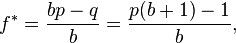
where:
- f* is the fraction of the current bankroll to wager;
- b is the net odds received on the wager (“b to 1?); that is, you could win $b (plus the $1 wagered) for a $1 bet
- p is the probability of winning;
- q is the probability of losing, which is 1 ? p.
As an example, if a gamble has a 60% chance of winning (p = 0.60, q = 0.40), but the gambler receives 1-to-1 odds on a winning bet (b = 1), then the gambler should bet 20% of the bankroll at each opportunity (f* = 0.20), in order to maximize the long-run growth rate of the bankroll.
If the gambler has zero edge, i.e. if b = q / p, then the criterion recommends the gambler bets nothing. If the edge is negative (b < q / p) the formula gives a negative result, indicating that the gambler should take the other side of the bet. For example, in standard American roulette, the bettor is offered an even money payoff (b = 1) on red, when there are 18 red numbers and 20 non-red numbers on the wheel (p = 18/38). The Kelly bet is -1/19, meaning the gambler should bet one-nineteenth of the bankroll that red will not come up. Unfortunately, the casino doesn’t allow betting against red, so a Kelly gambler could not bet.
The top of the first fraction is the expected net winnings from a $1 bet, since the two outcomes are that you either win $b with probability p, or lose the $1 wagered, i.e. win $-1, with probability q. Hence:

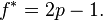
For even-money bets (i.e. when b = 1), the first formula can be simplified to:

Since q = 1-p, this simplifies further to
A more general problem relevant for investment decisions is the following:
1. The probability of success is  .
.
2. If you succeed, the value of your investment increases from  to
to  .
.
3. If you fail (for which the probability is  ) the value of your investment decreases from to
  . (Note that the previous description above assumes that a is 1).
In this case, the Kelly criterion turns out to be the relatively simple expression